Chapter10Residual Sum of Squares: Improving a Model’s Fit to Data
Goals
Use data from case reports to implement a method for estimating the value of the transmission parameter \(\beta\)
Understand how a “for” loop in Python helps us test many possible values of \(\beta\) with one click of the Evaluate button
Ensure that the results from our math-and-coding-based approach to estimating \(\beta\) make biological sense
So far, we have estimated \(\beta\) in two ways: (1) visually, making adjustments so that data and graphs are closer together, starting in Chapter 3, and (2) using a formula involving \(\mathcal{R}_0\) and parameters from our model, such as in (5.1) and (7.3), to substitute in values we could find from epidemiological information and solve for \(\beta\text{,}\) which is typically the only unknown value in the formula. In this chapter, we learn a new approach.
Begin in Exploration 10.1 by examining data points as well as values determined by an SI model. In this exploration, think about mathematical approaches to improve the model’s fit to data.
Exploration10.1.Visually Demonstrating Differences Between a Model and Data.
This example focuses on an SI model, similar to what we worked with in Chapter 2 and Chapter 3. Use the code shown, and its output, to answer the questions below.
(a)
Copy the graph from the Python output: draw it by hand or print it out if you prefer a paper copy, or create a digital version you can edit, such as a screenshot.
For the values \(I(0)\text{,}\)\(I(1)\text{,}\)\(I(2)\text{,}\)\(I(3)\text{,}\)\(I(4)\text{,}\)\(I(5)\text{,}\) and \(I(6)\) that are printed out in the Python output above the graph, label on your copy of the graph where each value is shown.
Then write out in words what the values \(I(0)\text{,}\)\(I(1)\text{,}\)\(I(2)\text{,}\)\(I(3)\text{,}\)\(I(4)\text{,}\)\(I(5)\text{,}\) and \(I(6)\) represent: are these data points, or values generated by a mathematical model?
(b)
Next, read lines 7 and 8 in the Python code.
These values combine to form several points on the output graph. On your copy of the graph, label the points determined by lines 7 and 8.
Then write out in words what the values from lines 7 and 8 represent: are these data points, or values generated by a mathematical model?
(c)
We now put parts (a) and (b) together.
Use your labeled graph to compare the values in part (a) with the values in part (b). Can you draw a visual way of comparing these values at each of the times \(t=0\text{,}\)\(t=1\text{,}\)\(t=2\text{,}\)\(t=3\text{,}\)\(t=4\text{,}\)\(t=5\text{,}\) and \(t=6\text{?}\)
Starting with the visual comparison you just described: What would change visually if the values from the model, and the values at each data point, were closer together?
Turn your visual comparison ideas into some mathematical suggestions for identifying when the model and the data are closer together.
Section10.1Residual Sum of Squares: An Introductory Example
One way to compare data with the output of a model is by computing the Residual Sum of Squares, often abbreviated as RSS. When we work with a single model to try to improve the fit of the model to a data set, RSS is a commonly used option. Activity 10.2 shows the steps for computing RSS for a model with one choice for a value of \(\beta\text{.}\) Then, Section 10.2 provides more mathematical context for how RSS works. After that, Section 10.3 shows how to compare RSS for different values of \(\beta\) used in the same model.
Activity10.2.
In Exploration 10.1 we worked with both a data set, and model output, for the Infectious population \(I(t)\) at times \(t=0, 1, 2, 3, 4, 5, 6\text{.}\) The data values and model output appear in Table 10.1, with model output rounded to two decimal places.
Table10.1.SI Model: Data Values and Model Output for \(I(t)\)
Time
Data Value
Model Output
0
1
1.0
1
2
4.19
2
4
14.54
3
10
32.38
4
22
44.58
5
40
48.68
6
50
49.70
RSS compares each Data Value from Table 10.1 with the Model Output from the same time by subtracting one from the other and squaring the result.
Try at least two of these comparisons on your own: for times \(t=1\) and \(t=2\text{,}\) subtract the Model Output in Table 10.1 from the corresponding Data Value and square the result. Later in this activity, we will compare these hand-computed values with the corresponding values computed via Python.
Read the code block below to identify where in the code, and how, we do each of the following. You may find it helpful to look up some of the Python commands online to better understand the details of how they work. Printing output is another way to build understanding: you can include commands such as print(sol) or print(t_range) near the bottom of the Python code block to be sure you understand the structures of sol, t_range, or other quantities.
The default code computes the numbers of Susceptibles and the numbers of Infectious at times 0, 0.1, 0.2, 0.3, and so on, until time 6.9. Where and how does the code say to do this?
When we say to complete a command for x in range(0,7), which values of \(x\) are we specifying?
Line 24 begins with for and then, in lines 25, 26, and 27, gives three commands. The word for means to complete these commands repeatedly, as many times as specified in the x in range(0,7) command you focused on in part (b) above. What happens in each of the three commands following for? For line 27, connect your answer back to the command RSS = 0 in line 22.
Within line 25, how do we specify that we seek Model Output at times 0, 1, 2, and so on, but not the Model Output at non-integer times such as 0.3? Why do we need to specify that we seek Model Output only at integer-valued times?
Run the code block. Compare its results with your results for \(t=1\) and \(t=2\) in part (1) of this Activity. Describe how the results are similar and how they are different, and provide an explanation for why they are not identical.
Then examine all the results from the code, including the total value for RSS for this model with this data set. State at least two of your observations.
Once you understand how the code works, experiment with different values of \(\beta\text{.}\) Your goal is to improve the fit between the model and the data set. While adjusting \(\beta\text{,}\) consider including a plot of the graph showing both the solution curve of the model and the data points. You can do this by copying plotting commands from the Python block in this chapter’s Exploration (lines 30 through 37) and pasting them into the bottom of the Python block in this activity.
Write about your experiments and their results. State how you improved the fit of the model to data by adjusting \(\beta\text{,}\) and include an explanation of how you know the fit is improved.
Answer.
At time \(t=1\text{,}\) compute \((4.19-2)^2\) to get the value \(4.7961\text{.}\) At time \(t=2\text{,}\) compute \((14.54-4)^2\) to get the value \(111.0916\text{.}\)
Line 20 tells Python to compute sol, which is the array of values of Susceptibles and Infectious at all times in t_range. Line 18 establishes t_range as the times from 0.0 to 6.9 using the command t_range = np.arange(0.0, 7.0, 0.1). Here, np.arange(0.0, 7.0, 0.1) indicates that the range of time values in t_range should start at time 0.0 and end at time 7.0, moving in time increments of 0.1. This means we compute solutions at times 0.0, 0.1, 0.2, and so on, with the last solutions computed at time 6.9. To see the values in t_range, you can run the Python block with the added command print(t_range). (We discussed these commands in Activity 3.4 and are refreshing our memory on them here.)
The command x in range(0,7) specifies the values \(x=0,1,2,3,4,5,6\text{.}\) In general, Python begins with, and includes, the first number in a range command, and then stops at, but does not include, the last number in the range command. This is why \(0\) is included, but \(7\) is not. To see the values in range(0,7), you can run the Python block with the added command for x in range(0,7): followed by the line print(x). The second line needs to be indented.
The command in line 25 starts with the Data Value given in line 8 by I_data[x] and subtracts the Model Output given by sol[10*x, 1]. The resulting value is then squared, and the squared value is given the name new_square.
The command in line 26 prints the value new_square computed in line 25. Printing pieces of output can help us make sure the code is doing what we expect and want it to do.
The command in line 27 updates the value of RSS by adding in the most recently computed value of new_square. Earlier in the code, in line 22, we set the value of RSS to 0. This makes certain that we always being with \(RSS=0\) and add only the squared distances for our current comparison of Data Values with Model Outputs.
We select Model Output values only at integer-valued time steps by multiplying x by 10 when writing sol[10*x, 1]. Recall that the array sol contains Model Output for \(S(t)\) and \(I(t)\) for \(t=0.0, 0.1, 0.2, 0.3, ..., 6.9\text{.}\) We select Model Output at times \(t=0.0, 1.0, 2.0, 3.0, 4.0, 5.0, 6.0\) to correspond to the times at which Data Values exist for comparison. Since x takes on values from \(0.0\) to \(6.9\text{,}\) and since Python counts starting at \(0\text{,}\) then sol[10*0, 1] tells us the Model Output at time \(0\text{,}\)sol[10*1, 1] tells us the Model Output at time \(1\text{,}\) and so on, until sol[10*6, 1] tells us the Model Output at time \(6\text{,}\) where \(6\) is the last time for which we have a Data Value.
The code produces the value \(4.795784246749833\) for the squared distance at time \(t=1\text{.}\) Our hand-computed value from part (1) of this Activity was \(4.7961\text{.}\) We see that these values are very close to each other. The difference between them is due to our rounding the values in Table 10.1 to two decimal points.
Similarly, the code produces the value \(111.02234652523701\) for the squared distance at time \(t=2\text{,}\) whereas our hand-computed value from part (1) of this Activity was \(111.0916\text{.}\) Again, the difference in values is due to rounding.
From here, make additional observations. This is open-ended. Observations may include noticing that the squared distances are notably larger when the data point is further from the value on the solution curve of the model, compared with when the data point is close to the value on the solution curve of the model. There may also be observations about the overall number computed for RSS. This overall RSS number is helpful when we reach part (4) and try to improve the fit of the model to data
Many other observations are possible.
This is open-ended. Values of \(\beta\) that are closer to \(0.02\) tend to produce a better fit of model to data, compared with the starting value of \(\beta = 0.03\text{.}\) You may wish to change additional decimal places of \(\beta\) to improve the fit even further.
It is also appropriate to give visual (graph-based) and verbal (word-based) descriptions of changes in the graph of model and data, as the value of \(\beta\) changes.
Section10.2The Underlying Math of RSS
This section first provides a visual demonstration of what we do when computing RSS, and then presents RSS as a mathematical formula. A goal of this book is for you to dive into modeling, often using examples as a first way to understand how you can build and analyze your own models. We therefore started with Activity 10.2, which showed RSS in an example-based way. Now, while describing the mathematical approach more formally, we regularly refer back to Activity 10.2.
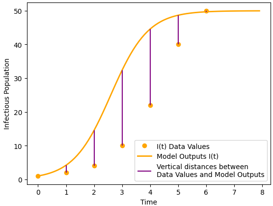
Start by considering Figure 10.2, which visualizes the subtraction that you did in Step 1 of Activity 10.2 and that the Python code did in line 25. Each subtraction takes the form of a purple vertical line. The length of each vertical line is the distance between the Model Output and the Data Value at a specific time \(t\text{.}\)
This graph shows Data Values as orange dots and Model Output as a smooth curve. The graph also shows the distances between Data Values and Model Output, at times \(t=0, 1, 2, 3, 4, 5, 6,\) for the SI model from Exploration 10.1, using \(\beta = 0.03\text{.}\)
Figure10.2.Graph showing distances between Data Values and Model Output for the SI model from Exploration 10.1, using \(\beta = 0.03\)
After computing vertical distances in Activity 10.2, we then square these distances. Take some time to think through the mathematical outcomes of squaring. One consequence of squaring each distance is that the results will always be non-negative, that is, either positive or zero. Throughout Activity 10.2 we start with the Data Value and subtract the Model Output, but we could have subtracted in either order because the results after squaring are the same. When we later add together all the squared differences, each vertical distance contributes in a positive way to the sum (or keeps the sum the same, if the vertical distance is zero).
Another aspect of squaring the distances is that a squaring function grows in an increasing way. This means that one large distance has the potential to contribute much more to the RSS value than several smaller distances. We can visualize this by thinking about the function \(y=x^2\text{.}\) Just as the \(y\) values on the graph of \(y=x^2\) increase much more rapidly than their corresponding \(x\) values, the squares of the distances increase much more rapidly than the distances themselves. The result is that larger distances can contribute to a vastly increased RSS value.
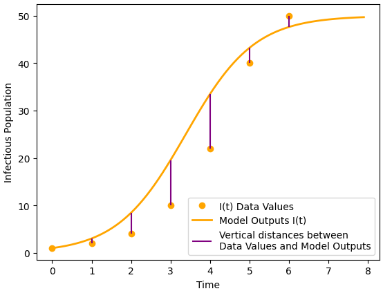
Next, turn to Figure 10.3 and notice that the Data Values are the same as in Figure 10.2, but the curve of Model Outputs grows more slowly. As a result, the vertical distances between Data Values and Model Outputs tend to be—but are not always—smaller. Previously, such as in Chapter 3, we relied only on trial and error, along with personal judgment, to estimate parameter values that would bring the model simulation closer to our data points. Now, the RSS formula both helps us bring the model closer to the data and, importantly, provides a metric by which we can measure that closeness.
This graph shows Data Values as orange dots and Model Output as a smooth curve. The graph also shows the distances between Data Values and Model Output, at times \(t=0, 1, 2, 3, 4, 5, 6,\) for the SI model from Exploration 10.1, using \(\beta = 0.023\text{.}\)
Figure10.3.Graph showing distances between Data Values and Model Output for the SI model from Exploration 10.1, using \(\beta = 0.023\)
Here are the steps for computing RSS for a specific mathematical model, with specific parameter values, in comparison with a particular set of data values.
Start by determining the Model Output at each time when we have a corresponding Data Value. In Activity 10.2, the Data Values occur at times \(t=0,1,2,3,4,5,6\text{,}\) so we use Model Output values for each of those times.
Notice that the Data Values and Model Outputs count the same things: the number of current Infectious individuals. In some other models, we will need to take additional steps to ensure that the quantities in our model relate directly to the quantities in our data set.
For each time \(t\text{,}\) subtract \((\mbox{Data Value at time }t - \mbox{Model Output Value at time }t)\text{.}\)
Compute the squares of each value you computed in the previous step. That is, for each time \(t\text{,}\) compute \((\mbox{Data Value at time }t - \mbox{Model Output Value at time }t)^2\text{.}\)
Add together all the squared values. The formula below relates to Activity 10.2, with Data Values at times \(t=0,1,2,3,4,5,6\text{.}\) In an example with different time values \(t\text{,}\) the summation may need to involve numbers other than the integers from \(0\) to \(6\text{:}\)
\begin{gather*}
\sum_{t=0}^{6} (\mbox{Data Value at time }t - \mbox{Model Output Value at time }t)^2 .
\end{gather*}
This formula allows us to compute RSS for each choice of \(\beta\) in our model. We then compare values of RSS for different choices of \(\beta\text{,}\) seeking the smallest RSS value among values of \(\beta\) that make sense biologically.
That last sentence deserves extra emphasis: it is crucial that \(\beta\) make sense biologically! Many modelers are tempted to minimize the RSS value in any way they can, losing sight of the biological importance of parameter values. We emphasize, throughout this book, that our model parameters have biological meaning, and therefore the values we choose for those parameters need to make real-world sense.
Section10.3Residual Sum of Squares: Quickly Comparing Multiple Parameter Values
As we saw in Section 10.1, we can bring model simulations closer to a data set by trying different parameter values, such as by allowing \(\beta\) to take on different values. In the Python code block within Activity 10.2, for every value of \(\beta\) we wanted to try, we had to change the value of \(\beta\) within the code and run the code again. Here, we instead wrap another for loop around the RSS for loop, so that we can test multiple values of \(\beta\) with one click of the Evaluate button.
Activity10.3.
This Activity focuses on coding, with the goal of comparing RSS values for multiple values of a parameter without having to run Python code separately for every value of that parameter. Start by reading the code in the Python block below, and use what you read to answer the questions that follow.
Describe how we gave a value to \(\beta\) in the code within Activity 10.2, compared with how we give values to \(\beta\) now in the code for Activity 10.3. State the lines of code in which \(\beta\) is given its values, and compare the commands used to give \(\beta\) its values, explaining how each command works.
In Activity 10.2 we run the command sol = odeint(hz, y0, t_range) and give RSS its initial value of \(0\) outside any for loop. Now, in Activity 10.3, we run odeint and reset RSS = 0 inside the new outer for loop, but before running the inner for loop to compute RSS for a specific value of \(\beta\text{.}\) Explain the reasoning for where in the code we run odeint and set RSS=0.
Discuss how indenting works for the nested for loops. Python requires correct indenting.
Discuss the commented-out print command in line 25. Why might we choose not to see these results in this code, whereas we wanted to see these results in Activity 10.2, where this command appeared on line 26? Then discuss the print command in line 27, and explain why the information it shows is especially helpful to us as we cycle through values of \(\beta\text{.}\)
Answer.
In Activity 10.2 we give \(\beta\) just one value, in line 16, by writing beta = 0.03, that is, by naming \(\beta\) and using the = sign to assign a value to \(\beta\text{.}\) The default code gives \(\beta\) the value \(0.03\text{,}\) and we can change this value by changing \(0.03\) to a different number.
In Activity 10.3 we state in line 19 that we will give \(\beta\) the values \(0.01, 0.02, 0.03, 0.04,\) and \(0.05\text{,}\) one at a time. The first time the for loop runs, \(\beta\) is given the first of this list of values, that is, \(\beta = 0.01\text{.}\) Each time the for loop runs, \(\beta\) is given the next value, as shown in line 20 of the code. In all, the default loop will run five times, once for each value of \(\beta\text{,}\) and \(\beta\) will take on each value one time. We can change the values in line 19 to run whichever values of \(\beta\) we like.
For each value of \(\beta\text{,}\) we use Python to do two things: solve the system of differential equations for that value of \(\beta\text{,}\) and compute the resulting RSS value comparing our Data Values with the Model Output from the solved differential equations. The outer for loop cycles through different values of \(\beta\text{.}\) For each, we recompute the solution array sol by running odeint on line 21, and we reset RSS = 0 on line 22. We are then ready to run the inner for loop, starting on line 23, where we compute the specific RSS value for the current value of \(\beta\text{.}\) It is important for computing this RSS value that we have reset RSS = 0 so that we do not add new squared differences to a past (non-zero) RSS value.
Python syntax requires that we indent the commands within a for loop. Indenting also serves as a visual signal to us, indicating which for loop each command is part of. The commands within the outer for loop, including the first line of the inner for loop, are indented the same amount. The commands within the inner for loop are indented further. Notice that the print command on line 27 is not as indented as commands on lines 24, 25, and 26. This tells us that line 27 is part of the outer for loop rather than the inner for loop.
The print command from line 25 was especially helpful in Activity 10.2 when we were learning, and perhaps troubleshooting, the code for computing RSS for a specific value of \(\beta\text{.}\) In Activity 10.2 this print command appeared in line 26, and it showed us the step-by-step squared distances computed in Python that would be added together to produce the total RSS value. We compared some of these squared distances with values we computed by hand, both to make sure Python was doing what we wanted, and to build student understanding of the meaning of the RSS value.
Once we understand how this for loop works when computing RSS, we do not usually need to print all the squared distances. This is the reason why the print command in line 25 of the code for Activity 10.3 is commented out. We can use this code if we want by removing the # at the start of the line, but now we are more focused on seeing the RSS results for each value of \(\beta\text{.}\) These RSS results appear due to the print command in line 27, and we compare them to determine which \(\beta\) values produce the smallest values for RSS.
For Further Thought10.4For Further Thought
1.
The paper Outbreak of 2009 Pandemic Influenza A (H1N1) at a New York City School describes a high school outbreak from April 2009. 1
The article appears in the New England Journal of Medicine in Volume 361, published in 2009, pages 2628-2636. The authors are Justin Lessler, Nicholas G. Reich, Derek A.T. Cummings, and the New York City Department of Health and Mental Hygiene Swine Influenza Investigation Team. Here is a link to the article: https://www.nejm.org/doi/full/10.1056/NEJMoa0906089.
Data from the outbreak, along with 2-day prevalence data computed as in Chapter 9, appear in Table 10.4. We use only two days for prevalence because people with flu symptoms typically stay home. This model, therefore, supposes they may go to school briefly while feeling sick, but then they stay home and no longer spread the illness to others at the school.
Table10.4.H1N1 Influenza Data from a New York City High School, 2009
Date (Day)
New Cases
2-day Prevalence
April 18 (Day 0)
23
23
April 19 (Day 1)
10
33
April 20 (Day 2)
17
50
April 21 (Day 3)
23
73
April 22 (Day 4)
103
176
April 23 (Day 5)
267
420
April 24 (Day 6)
147
557
April 25 (Day 7)
100
640
April 26 (Day 8)
50
667
April 27 (Day 9)
17
581
April 28 (Day 10)
7
321
April 29 (Day 11)
7
181
April 30 (Day 12)
7
88
May 1 (Day 13)
3
41
Use Python to plot the 2-day prevalence data.
Construct an SIR model with isolation, in the style of Figure 8.2, with parameter values for this outbreak. Use in your model the information that the population is 2934 people (students plus employees) and the infectious period was 2 days (to match the 2-day prevalence assumption). Implement an RSS approach to select a preferred value of \(\beta\text{.}\)
Include your Python code, and show at least three different values of \(\beta\) that you tried, along with the corresponding RSS value for each value of \(\beta\text{.}\) Then state your selected value of \(\beta\) and graph the 2-day prevalence Data Values on the same axes as the Model Output, that is, the \(I(t)\) graph produced by using your selected value of \(\beta\text{.}\)
Discuss your results from part (b). Qualitatively, how well does the \(I(t)\) curve fit the Data Values when you use your selected value of \(\beta\text{?}\) Consider how rapidly the \(I(t)\) curve increases and decreases, and the height and timing of when the 2-day prevalence curve peaks.
The value of \(\mathcal{R}_0\) for H1N1 has been estimated to be between 1.4 and 1.6, and a typical length of infectiousness for H1N1 is 5 days. Using (5.1) and \(N=2934\text{,}\) what value of \(\beta\) would result from this information? How close is the value of \(\beta\) you selected using RSS to the range of values of \(\beta\) that make sense in (5.1)? Discuss possible reasons for the outcome you find, whether you found that the \(\beta\) values are close or not very close.
2.
Work through Exercise 1, above, one more time, supposing instead that people come to school just one day during the time they are infectious with influenza. This means setting up a model using the New Cases values in Table 10.4 rather than the 2-day Prevalence values.
Then compare your results with what you found in Exercise 1. Based on what you found in your models, and also based on any real-life experience you may have with flu outbreaks, what do you see as the advantages and disadvantages in each version of the model?
3.
As described starting on page 356 of Mathematical Models in Population Biology and Epidemiology, second edition, by Fred Brauer and Carlos Castillo-Chavez, the village of Eyam, in England, was affected by bubonic plague in 1665-1666. There were two separate plague outbreaks, and Table 10.5 shows data for the second of these outbreaks.
Table10.5.Plague Data from Eyam, 1666
Date (Day)
Susceptibles
Infectious
July 3/4 (Day 0)
235
14.5
July 19 (Day 15.5)
201
22
August 3/4 (Day 31)
153.5
29
August 19 (Day 46.5)
121
21
September 3/4 (Day 62)
108
8
September 19 (Day 77.5)
97
8
October 4/5 (Day 93)
Unknown
Unknown
October 20 (Day 108.5)
83
0
Use Python to plot these data.
Then, use the information that we start with a population of 250 people, the infectious period was 11 days, and \(\mathcal{R}_0\) has been estimated to be between 1.6 and 1.9, to construct an SIR model for this outbreak.
Then use an RSS approach, along with the data and your SIR model, to select a preferred value of \(\beta\) for this SIR model. There are two new and different details to attend to.
The data from October 4/5 are Unknown. You may choose to address only the six preceding dates, or to also include the data from October 20. State which data points you are including in your RSS calculation.
The dates in this example are 15.5 days apart, rather than 1 day apart. This requires changing the 10 in the sol[10*x, 1] part of the Python code.