This textbook has focused, so far, on models of outbreaks. In each model, a disease has emerged, then peaked, then faded away. Yet many diseases remain in a population over a long period of time, passing from person to person in such a way that the disease remains in the population across many years. This chapter addresses such diseases.
Begin in Exploration 11.1 by using the skills you have been developing to think about how you might construct two different types of model showing endemic illness, that is, an illness that remains in a population long-term rather than peaking and fading.
Exploration11.1.A Disease that Remains Long-term in a Population.
Think through each of the following scenarios. Use your experience building compartmental models to develop a compartmental model for each of the new scenarios described.
Assume a disease has Susceptible, Infectious, and Removed phases, and that people in the Removed compartment lose immunity over time. These people then go back to the Susceptible compartment. This ongoing renewal of the Susceptible population allows the disease to last beyond just an initial peak of infectious people. Draw a possible compartmental diagram and differential equations for such a model, and draw a graph sketching how the long-term population values might look. This exploration is not asking you to develop Python code to draw the graph, but instead to hand-draw your best guess.
Next, assume a disease has Susceptible, Infectious, and Removed phases, and that people in the Removed compartment do not lose immunity over time. Instead, new people enter the Susceptible compartment due to births or immigration, and people depart all three compartments due to deaths or emigration. Draw a possible compartmental diagram and differential equations for such a model, and draw a graph sketching how the long-term population values might look. This exploration is not asking you to develop Python code to draw the graph, but instead to hand-draw your best guess.
Section11.1Comparing Endemic Illnesses with Epidemics
This chapter focuses on models of endemic illness. By contrast, so far this semester, we have studied epidemic illnesses, also called epidemics or outbreaks. With epidemics, the Infectious population reaches its peak, drops to 0, and the epidemic ends. With endemic illness, the illness persists over time in the population.
A wording note: while we may refer to “an epidemic”, we never refer to “an endemic”. Instead, we can talk about “endemic illness” or “endemic disease”: the word “endemic” always describes something, but “endemic” does not refer to the event itself.
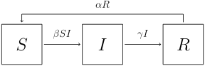
Consider the compartmental diagram shown in Figure 11.3, depicting an illness in which people in the Removed compartment can lose immunity and return to the Susceptible compartment. Use the questions below the diagram to think through the details of this model.
The compartmental diagram for an SIRS model, having compartments for populations of Susceptible, Infectious, and Removed or Recovered people. Arrows point from S to I, from I to R, and from R to S.
Sometimes the R compartment in a model includes only people who have recovered from illness, meaning the R could stand for Recovered. Alternatively, sometimes the R compartment includes recovered people as well as others, such as those who have died, in which case we typically say that R stands for Removed. Write a reasonable interpretation for the R compartment shown in Figure 11.3.
Graph each model’s solution curves \(S(t)\text{,}\)\(I(t)\text{,}\) and \(R(t)\) in Python. Start with the default parameter and initial values in the Python code below, including time ending at \(t=30\text{.}\)
What seems to be happening when you stop at \(t=30\text{?}\) In order to better understand the long-term behavior of the system, what is a good end time \(t\text{?}\) When responding to this question, change just the end time, not any other values.
The formula \(\alpha R\) describes movement from the R compartment to the S compartment. The value of \(\alpha\) indicates how quickly people move from R to S.
In this model, people enter the S compartment from the R compartment, unlike in, say, the SIR model from Figure 4.4, where people can only depart the S compartment. This means the S population may decrease less quickly, or can remain at some nonzero population value, or can increase. These possibilities mean we may not run out of Susceptibles as a way of ending the illness, so it is possible for the Infectious compartment to never reduce to 0 people.
While we could still call the R compartment “Removed”, it may be more precise to say that R here means “Recovered”. This indicates that everyone in the R compartment has recovered from illness and is still alive, which is important when we say that people in the R compartment are able to move to the Susceptible compartment where they may be infected again.
At \(t=30\text{,}\)\(S(t)\) has dipped but is rising, whereas \(I(t)\) and \(R(t)\) have risen and appear to be falling. Running the model for a longer time shows that the curves appear to level out to horizontal by about \(t=40\text{.}\) It helps to show the model for longer than this, to \(t=50\) or somewhat longer, to be sure the curves stay horizontal.
The primary change in Activity 11.2, as compared with the SIR model we have studied previously, is that people from the R compartment can return to S. This change to the model can mean that we never run out of people in the S compartment or in the I compartment. For this reason, the illness can last forever in the population.
The value of \(\alpha\) can be determined by how long people typically stay in the R compartment. This is similar to how we have determined the value of \(\gamma\text{,}\) such as in (4.1) and (4.2), and the value of \(\kappa\text{,}\) such as in (7.1) and (7.2).
There is another typical way for an illness to remain endemic in a population. Continue on to Activity 11.4 to learn about and experiment with such a model.
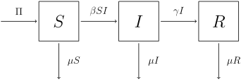
Now consider the compartmental diagram shown in Figure 11.5, depicting an infectious illness in a population where people enter and exit the population. Use the questions below the diagram to think through the details of this model.
The compartmental diagram for an SIR model with demographics, having compartments for populations of Susceptible, Infectious, and Removed or Recovered people. Arrows point from S to I and from I to R. An arrow points into S from the outside, and arrows point out from all three compartments.
This model allows people to enter the population by births or immigration, and allows people to leave the population by deaths or emigration. Comment on what this may mean for the timespan of such a model, in comparison with the timespan of an outbreak model in which we leave out these options for people to enter or exit the population. That is: how long, in terms of weeks, months, or years, might you expect this sort of model to last, compared with an outbreak model lacking demographic changes?
Graph each model’s solution curves \(S(t)\text{,}\)\(I(t)\text{,}\) and \(R(t)\) in Python. Start with the default parameter and initial values in the Python code below, including time ending at \(t=50\text{.}\)
What seems to be happening when you stop at \(t=50\text{?}\) What if you go to \(t=500\text{?}\) What if you go to \(t=5000\text{?}\) In order to better understand the long-term behavior of the system, what is a good end time \(t\text{?}\) When responding to this question, change just the end time, not any other values.
The formula \(\Pi\) indicates that people enter the S compartment at some constant rate. The formulas \(\mu S\text{,}\)\(\mu I\text{,}\) and \(\mu R\) indicate that people leave the S, I, and R compartments at a rate proportional to how many people are in those compartments. These formulas also show that in this model, the proportion of people leaving each compartment is the same proportion, rather than different proportions for different compartments.
In this model, people enter the S compartment due to births or immigration, unlike in, say, the SIR model from Figure 4.4, where people can only depart the S compartment. This means the S population may decrease less quickly, or can remain at some nonzero population value, or can increase. These possibilities mean we may not run out of Susceptibles as a way of ending the illness, so it is possible for the Infectious compartment to never reduce to 0 people.
A model involving births and deaths, or immigration and emigration, has the capacity to last much longer than a model lacking these terms. For an outbreak lasting a few weeks or months, we typically leave these terms out because any changes from them are negligible over a short time. Including them usually means our timeframe is longer, so that we cannot meaningfully leave them out.
At \(t=50\text{,}\) the results appear similar to those in many SIR models we have seen. The \(I(t)\) curve has peaked and fallen to nearly 0, the \(S(t)\) curve has dropped, and the \(R(t)\) curve has risen. It is worth noticing, though, that the \(S(t)\) curve has not fallen to 0, but seems to end in a nearly horizontal line at a value of approximately 800 people.
Extending to \(t=5000\text{,}\) things get very interesting. The \(S(t)\) and \(R(t)\) populations oscillate over time, while \(I(t)\) shows occasional brief peaks. It appears that the populations may be leveling out near the end of the time shown in the graph. Letting the graph run until \(t=8000\) or \(t=10000\) further suggests that the populations reach long-term equilibrium values at which none of the populations goes to 0. (The scale of the graph may make it seem as though \(I(t)\) approaches 0, but we can print long-term population values to see that \(I(t)\) approaches approximately 33.)
(The scale of the graph may make it seem as though \(I(t)\) approaches 0, but we can print long-term population values to see that \(I(t)\) approaches approximately 33. To print this value, add a line near the bottom of the Python code saying print("Long-term value of I = ", round(sol[-1,1])).)
We have now seen two distinct ways to model endemic illness. In Activity 11.2 the Susceptible population is replenished as people leave the R compartment and return to S. This allows the illness to continue, cycling through the population, meaning that individuals can become sick more than once. In Activity 11.4 the Susceptible compartment gains people through births or immigration, which is a different way to maintain a population that can be infected. Indeed, many so-called “childhood illnesses” in history have lasted so long because there are always new children in the population who have not yet contracted the illness and therefore are not yet immune. This is why these illnesses mostly occur in children, often very young children.
It is also possible to have a model combining the concepts from Activity 11.2 and Activity 11.4, that is, a model can have demographic changes and also allow Recovered people to lose immunity and return to the Susceptible compartment. Yet another possibility is to set a different death rate in the Infectious compartment, if an illness can lead to death. In this case, the death rate for the I compartment should be larger than the death rates for the S and R compartments.
Mathematically, models of endemic illness have the interesting outcome that we can compute equilbrium values for a long-term outcome in which disease remains in the population. As the models become more complicated, we may not try to compute these equilbrium values as algebraic formulas, but instead we see them in simulations. Notice, for example in Activity 11.2 and Activity 11.4, that the equilibrium values are the values of each population as the solution curves became horizontal, at nonzero values, when the model runs for a long time.
In Section 11.2 we show how to compute equilbrium values for the relatively simple models of endemic illness that we have been exploring in this section.
Section11.2Equilibrium Values in Endemic Illness Models
This section focuses on equilibrium values. In a compartmental model, equilibrium occurs when each compartment maintains an unchanging population. For an SIR model, equilibrium means that \(dS/dt = 0\text{,}\)\(dI/dt = 0\text{,}\) and \(dR/dt = 0\text{.}\)
You may notice that any compartmental model could be at equilibrium if the total population size were 0. Consider, for instance, the Activity 11.2 model
In this model, if we had \(S=0\text{,}\)\(I=0\text{,}\) and \(R=0\text{,}\) then the right-hand sides of each equation would equal 0, which means that each derivative would equal 0. It is completely accurate to notice this form of equilbrium, yet it does not tell us much about disease spread in a population containing any people. So, we note it and move on.
Another type of equilibrium is a disease-free equilibrium. We consider this as the equilibrium for a disease model in a population that has not yet encountered the disease. Prior to disease arrival, \(I=0\) and \(R=0\text{.}\) In our models for Activity 11.2 and Activity 11.4, disease-free equilibrium means that the entire population is in the S compartment. When we define \(N=S+I+R\text{,}\) meaning that \(N\) represents the entire population, then the disease-free equilibrium has \(S=N\text{,}\)\(I=0\text{,}\)\(R=0\text{.}\)
The activities below focus on yet another equilibrium, namely the endemic equilibrium. The epidemic models we have studied could not have such an equilibrium because disease would invariably peak and then recede. With endemic illness, there can be a long-term state in which \(I \neq 0\) and \(R \neq 0\text{.}\) This is the type of equilibrium we will solve for algebraically and then study, beginning with Activity 11.6.
In this activity, we solve algebraically for the endemic equilibrium \((\overline{S}, \overline{I}, \overline{R} )\) of the compartmental model shown in Figure 11.3. The lines atop \(S\text{,}\)\(I\text{,}\) and \(R\) indicate that these are the specific values of each compartment’s population for which the entire system is at equilibrium. To help us start the algebra needed to compute the formulas we seek, we use the knowledge that at equilibrium all three differential equations from the model in Activity 11.2 are set equal to 0, indicating that the values are unchanging for all three populations \(S(t)\text{,}\)\(I(t)\text{,}\) and \(R(t)\text{.}\) Here are the expressions that result when we set the derivatives of the model equal to 0:
Solve (11.3) for \(S\text{.}\) In other words, rearrange \(\beta SI - \gamma I=0\) into an equation beginning with “\(S=\)” and having only non-\(S\) terms on the right-hand side. Your result can also be written as \(\overline{S}\text{.}\)
Start with (11.2) and replace \(R\) with \(N-S-I\text{.}\) Explain why this is a permissible substitution. Then solve for \(I\text{.}\) Your answer will be in terms of \(S\text{,}\) which we solved for in part (1). Your result can also be written as \(\overline{I}\text{,}\) with \(S\) on the right-hand side written as \(\overline{S}\text{.}\)
Solve (11.4) for \(R\text{.}\) Your answer will be in terms of \(I\text{,}\) which we solved for in part (2). Your result can also be written as \(\overline{R}\text{,}\) with \(I\) on the right-hand side written as \(\overline{I}\text{.}\)
Your result should be three algebraic formulas giving equilibrium values \(\overline{S}\text{,}\)\(\overline{I}\text{,}\) and \(\overline{R}\) for the three populations in the model, entirely in terms of the parameter values \(\alpha\text{,}\)\(\beta\text{,}\) and \(\gamma\text{,}\) as well as the total population size \(N\text{.}\)
Be sure to show your algebra steps. Then, we could substitute in \(\overline{S}=\gamma / \beta\) to obtain a formula that is entirely in terms of the model’s parameters and the total population value.
Be sure to show your algebra steps. Then, we could substitute in the formula for \(\overline{I}\text{,}\) and within that substitute the formula for \(\overline{S}\text{,}\) to obtain a formula that is entirely in terms of the model’s parameters and the total population value.
Modeling involves many skills, from the algebra in Activity 11.6 to experimenting with simulations and their resulting numbers and graphs that help us build our understanding of how a particular model works. Continue to develop your understanding of the SIRS model from Figure 11.3 by completing Activity 11.7.
In Activity 11.6 we computed a formula for the endemic equilibrium value of the SIRS compartmental model shown in Figure 11.3. Next, we visualize solutions for this model using different parameter values, and for different amounts of time, and we compare these solutions with the equilibrium values determined by the formulas found in Activity 11.6.
Begin by reading the code carefully. Lines 17 through 20 define total population size \(N\) and starting values for each compartment’s population, with the starting value of \(I\) depending on the starting values of \(S\) and \(R\text{.}\) Then, on line 21, the vector y0 of starting values uses the values defined on lines 17 through 20. Explain how this way of writing initial population values and the vector y0 can help us quickly change these initial values as we try different simulations of this SIRS model.
Lines 23-25 of the code define S_equilibrium, I_equilibrium, and R_equilibrium. Explain where these formulas originated. Your answer should refer to Activity 11.6.
In lines 29-36 of the code, we print both end-of-simulation values of each compartment’s population, and the equilibrium values for those populations, for the simulation we have just created. With the default Python code provided, these values do not necessarily match very closely. First: explain clearly which three of the six printed values relate directly to the graph produced by Python, and explain the way they relate. Then state at least one reason why the end-of-simulation values do not match closely with the equilibrium values, and describe something you could change in the simulation to improve the match.
Make the change you described in (3) and report on the outcome. Detail the ways the end-of-simulation values and the equilibrium values match better, or if they do not match better, explain why you believe this is the case.
This is open-ended: there could be several possible answers. One likely answer is that listing initial conditions in this way means we can change just S_start and then I_start and the vector y0 change automatically, with the total population size \(N\) left (purposefully) unchanged.
Lines 23-25 of the Python code use the formulas we solved for in Activity 11.6 to directly compute equilibrium values for the \(S\text{,}\)\(I\text{,}\) and \(R\) populations.
The end-of-simulation values are those that relate to the graph. The end-of-simulation value of S gives the height of the \(S(t)\) graph at the end of the simulation, that is, at \(t=30\text{.}\) Similarly, end-of-simulation value of I gives the height of the \(I(t)\) graph at \(t=30\text{,}\) and end-of-simulation value of R gives the height of the \(R(t)\) at \(t=30\text{.}\)
Although the graphs seem to be getting close to long-term equilbrium values, they do not yet appear completely horizontal. This is a likely reason for the end-of-simulation values and the equilibrium values to not quite match. We should try to run the simulation for a longer amount of time to see if the model appears to reach its equilibrium and if, therefore, this match improves.
Running the simulation for a longer amount of time should work. Students should report how long they ran the model, how well the end-of-simulation values and the equilibrium values match, and any other observations that appear relevant.
Finally, return to the SIR model with demographics from Figure 11.5. The steps for computing the endemic equilibrium for this model appear in the first exercise of For Further Thought 11.3. In Activity 11.8, experiment with the graph of long-term solution curves and the printed values of the \(S(t)\text{,}\)\(I(t)\text{,}\) and \(R(t)\) values at the end of the simulation. By creating a variety of simulations and thinking through their results, you are building your knowledge and intuition for the dynamics of this model, which behaves in notably different ways than the model in Activity 11.7.
In a process similar to what we did in Activity 11.7, we visualize a variety of solutions for a model and compare these solutions with formulas for the equilibrium values of each compartment. Our focus model in this activity is the SIR model with demographics that we first saw in Activity 11.4.
Begin by reading the code carefully. State, by line number, where in the code the initial population values are established. Then state where in the code the formulas for the equilibrium values \(\overline{S}\text{,}\)\(\overline{I}\text{,}\) and \(\overline{R}\) are written, again using line number. Write, by hand, the equilibrium value formulas, writing the Greek letters rather than spelling them out as the code does. For example, write “\(\beta \,\)” rather than writing the letters “b”, “e”, “t”, “a”.
Notice that this model includes people entering and leaving the population, in a way that none of our previous models in this textbook have done. As a result, total population size \(N\) may not be constant. Solve here for the equilibrium value \(\overline{N}\text{,}\) where \(\overline{N}=\overline{S}+\overline{I}+\overline{R}\text{.}\)
To solve for \(\overline{N}\text{,}\) start with the differential equations for the SIR model with demographics. You developed these differential equations in Activity 11.4. Add together the three equations, and use your calculus-based knowledge of derivative rules to explain why, on one side, the sum becomes the following:
The other side of the summed differential equations should simplify to a small number of terms. Set this simplified expression equal to \(0\text{,}\) since \(dN/dt=0\) at equilibrium. Then use the definition \(N=S+I+R\) to introduce \(N\) into the equation and solve for \(N\text{.}\) The expression you create is the equilibrium value \(\overline{N}\text{.}\)
Finally, compute the value of \(\overline{N}\) for the default parameter values shown in the Python code, and compare \(\overline{N}\) with the initial population size N_start shown in the code.
In lines 30-37 of the code, we print end-of-simulation values of each compartment’s population for the simulation we have just created, as well as the equilibrium values for those populations. With the default Python code provided, these values do not match very closely. Activity 11.7 asks for your explanation for why these values may not match, and the reasons you provided there continue to be true in the SIR model with demographics. Now: state reasoning about \(\overline{N}\) differing from the initial total population value N_start to explain why the end-of-simulation values for each population do not match the equilibrium values.
Include the following two lines of code after line 37 to print the end-of-simulation value for \(N\) and the equilibrium value \(\overline{N}\text{.}\)
Run the code for the default 50 time steps, and for 500, 5000, and 8000 time steps. Use both printed Python output and the graphs you produce to demonstrate the long-term trend of the model to approach its equilibrium values \(\overline{S}\text{,}\)\(\overline{I}\text{,}\)\(\overline{R}\text{,}\) and \(\overline{N}\text{.}\)
Try additional experiments in which the starting values \(N\) are equal to, larger than, and smaller than the equilibrium value \(\overline{N}\text{.}\) Report on your results.
Initial population values N, S_start, R_start, and I_start are defined in lines 18-21. In line 22, the code forms these values into the vector y0 of initial values for the \(S\text{,}\)\(I\text{,}\) and \(R\) populations.
By the rules of calculus and derivatives, the sum of derivatives equals the derivative of a sum. That is, we can add the derivatives \(dS/dt\text{,}\)\(dI/dt\text{,}\) and \(dR/dt\text{,}\) or we can first add \(S+I+R\) and then compute the derivative \(d(S+I+R)/dt\text{,}\) and the answers will be the same. Since \(S+I+R=N\text{,}\) then we know that both \(dS/dt+dI/dt+dR/dt\) and \(d(S+I+R)/dt\) equal \(dN/dt\text{.}\)
Use the expression \(\overline{N}=\Pi /\mu\) from part (2) above to determine what the equilibrium population \(\overline{N}\) should be. Compare this with the initial population size N_start and the value of \(N\) at the end of the simulation, that is, after 50 time steps. You will see that the initial population size N_start is smallest, the population size at \(t=50\) is larger, and the equilibrium population \(\overline{N}\) is notably larger than both. This means that at \(t=50\) we are not yet close to the model’s equilibrium value.
Responses here are somewhat open-ended. Each should show outcomes of multiple simulations, each having a different number of time steps. Solutions should also show a trend that indicates that as the length of time for the simulation increases, the model appears to be reaching an equilibrium. Supporting evidence for reaching equilibrium should include both the numbers Python prints out and the behavior shown in the graphs Python produces.
This concludes our focus on models of endemic illness. Allowing populations to replenish their Susceptibles, through losing immunity or via people entering and leaving the population, significantly expands the types of illnesses we are able to represent with compartmental models. As we are nearing the end of Part I, the Core Modeling Concepts portion of this text, this is a good moment to think through the variety of modeling approaches we have seen and continue to build. Moving forward, we can combine these approaches into yet new models, with compartments and arrows selected to best represent the dynamics of outbreaks for which we develop the models ourselves.
Show the steps for how to solve algebraically for the endemic equilibrium \((\overline{S}, \overline{I}, \overline{R} )\) of the SIR model with demographics as shown in Figure 11.5. Start by setting equal to 0 the differential equations for the model:
\begin{align}
\Pi - \beta SI - \mu S \amp = 0 \tag{11.5}\\
\beta SI - \gamma I - \mu I \amp = 0 \tag{11.6}\\
\gamma I - \mu R \amp = 0 \text{.}\tag{11.7}
\end{align}
This indicates that the values are unchanging for all three populations \(S(t)\text{,}\)\(I(t)\text{,}\) and \(R(t)\text{.}\) Then follow the steps below.
Substitute \(\overline{S}\) into (11.5). Show how you do this. Then solve for \(I\text{,}\) showing your algebra steps to do so. This result is the equilibrium value \(\overline{I}\text{.}\)
Solve (11.7) for \(R\text{,}\) showing your algebra steps. The result contains \(I\text{.}\) When \(I=\overline{I}\text{,}\) this formula is the equilibrium value \(\overline{R}\text{.}\)
Your result should be three algebraic formulas giving equilibrium values for the \(S\text{,}\)\(I\text{,}\) and \(R\) populations, entirely in terms of the parameter values \(\beta\text{,}\)\(\gamma\text{,}\)\(\mu\text{,}\) and \(\Pi\text{.}\)
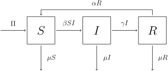
Follow the steps below to show how to solve algebraically for the endemic equilibrium \((\overline{S}, \overline{I}, \overline{R} )\) of the SIRS model with demographics as shown in Figure 11.9.
The compartmental diagram for an SIRS model with demographics, having compartments for populations of Susceptible, Infectious, and Removed or Recovered people. Arrows point from S to I, I to R, and R to S. An arrow points into S from the outside, and arrows point out from all three compartments.
Write out the equation that results when you set \(dI/dt=0\text{.}\) Then solve for \(S\text{,}\) showing your algebra steps along the way. This result is the equilibrium value \(\overline{S}\text{.}\)
Write out the equation that results when you set \(dS/dt=0\text{.}\) Substitute in \(R=N-S-I\) and the equilibrium value for \(S\) you computed in step (b) above, writing the formula with these substitutions. Then solve for \(I\text{,}\) showing your algebra steps for doing so. This result is the equilibrium value \(\overline{I}\text{.}\)
Write out the equation that results when you set \(dR/dt=0\text{.}\) Then solve for \(R\text{,}\) showing your algebra steps. The result contains \(I\text{.}\) When \(I=\overline{I}\text{,}\) this formula is the equilibrium value \(\overline{R}\text{.}\)
Your result should be three algebraic formulas giving equilibrium values for the \(S\text{,}\)\(I\text{,}\) and \(R\) populations, entirely in terms of total population size \(N\) and the parameter values \(\alpha\text{,}\)\(\beta\text{,}\)\(\gamma\text{,}\)\(\mu\text{,}\) and \(\Pi\text{.}\)
Set four or more values of \(\alpha\text{,}\) keeping \(\alpha\) in the range \(0.001 \lt \alpha \lt 0.9\text{.}\) (It is possible for \(\alpha\) values to extend beyond this range in reality, as long as \(\alpha \geq 0\text{.}\)) Describe the long-term behavior of the model for each of the \(\alpha\) values you choose. Be sure to confirm that your simulation runs long enough to approach its equilibrium: if any of the lines \(S(t)\text{,}\)\(I(t)\text{,}\) or \(R(t)\) do not appear horizontal near the end, or if any of the end-of-simulation population values are not close to their equilibrium values, then run the model for a longer time.
In Activity 11.8 we determined a formula for the equilibrium value \(\overline{N}\) for the total population. The same formula for \(\overline{N}\) shows the equilibrium population for the model in this exercise. State this formula, and run the model simulation at least three times, starting with initial population size \(N\) (i) smaller than, (ii) equal to, and (iii) larger than the equilbrium value \(\overline{N}\text{.}\) In each case, run the model for long enough to approach equilibrium. Describe what you see in each of the three cases, and make comparisons across the three cases.
Parts (a) and (b) in this exercise each provide experiments to run on the model from Figure 11.9. In part (c), develop another experiment. State your experiment, run it, and describe your results.